Whenever you go to the bank to deposit some cash money, the cashier places banknotes in a machine that tells whether a banknote is real or not. This is a classification problem where we are given some input data and we have to classify the input into one of the several predefined categories. Rule-based as well as statistical techniques are commonly used for solving classification problems. Machine learning algorithms fall in the category of statistical techniques.
Authenticating whether a banknote is real or not is one of the most common tasks in the banking industry.
In this article, we explain the process of building a banknote authentication system using machine learning algorithms. After reading this article, you will be able to understand how classification systems are built using machine learning algorithms.
The Need for Dataset
Machine learning algorithms learn from the dataset. Statistical algorithms are used behind the scenes to make a machine learning model learn from the data. Therefore, to identify whether a banknote is real or not, we needed a dataset of real as well as fake bank notes along with their different features. Luckily, we found such dataset at UCI Machine Learning repository, which is a repository of freely available datasets.
We used Python libraries for the analysis of our dataset as well as for training the machine learning models. To import the dataset we used the Pandas library. For visualizing the dataset we used Searborn library and finally to train machine learning algorithms we used Scikit learn library.
Note: All the Python scripts in this article have been executed using the Jupyter Notebook
Importing Required Libraries
Before we can import our dataset and perform analysis, we need to import a few libraries. The following script is used to import libraries:
import pandas as pd

import numpy as np

import seaborn as sns
In the script above, we import Pandas, Numpy and the Seaborn libraries.
Loading the Dataset
Once we import the libraries, the next step is to load the dataset into our application. To do so, we used the "read_csv()" function of the Pandas library, which reads dataset that is in the CSV format. The banknote dataset in CSV version can be found at this Github link.
The following script loads the dataset into “banknote_dataset” data frame:
banknote_datadset = pd.read_csv('https://raw.githubusercontent.com/
Kuntal-G/Machine-Learning/master/R-machine-learning/data/
banknote-authentication.csv')
Data Analysis
To see how the dataset actually looks, we can use the "head()" function of the Pandas data frame:
banknote_datadset.head()
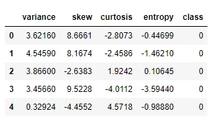
The "head()" function returns the first five rows of the dataset as shown below:
It is evident from the output that our dataset has four features: variance, skew, curtosis and entropy. While the class refers to whether or not the banknote is real or not.
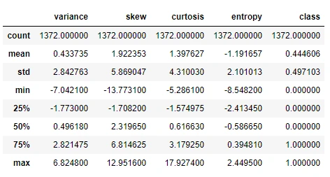
To see the statistical details of the data, the "describe()" function can be used, which returns the mean, count, standard deviation, quartile information and maximum values for each column.
banknote_datadset.describe()
The output shows the statistical information of the dataset. The dataset contains 1372 records.
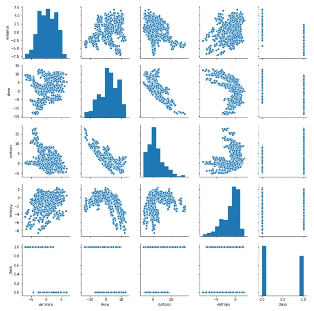
As a last data analysis step, we wanted to see the relationship between the different features in our dataset. To do so, we used the "pairplot()" function from the Seaborn library. The function takes dataset as a parameter and plots a graph that contains relationships between all the features in the dataset as shown below:
sns.pairplot(banknote_datadset)
It is visible from the output that entropy and variance have a slight linear correlation. Similarly, there is an inverse linear correlation between the curtosis and skew. Finally, we can see that the values for curtosis and entropy are slightly higher for real banknotes, while the values for skew and variance are higher for the fake banknotes.
Data Preprocessing
After the analysis phase, we needed to preprocess the data and convert it into a format that can be used to train machine learning algorithms.
In this regards, we performed two tasks.
1. Divide the Data into Features and Labels
Machine learning algorithms require data where features and labels are separated from each other. The label means the output class or output category. In our dataset, variance, skew, curtosis, and entropy are features whereas the class column contains the label. The following script divides data into features and labels sets.
dataset_features = banknote_datadset.iloc[:, 0:4].values

dataset_labels = banknote_datadset.iloc[:, 4].values

The "iloc" function takes the index that we want to filter from our dataset,
in the first line we filtered column 0 to column 3 that contain our feature set.
In the second row, we only filtered records from column four which contains the
labels (class).
2. Divide the Data into Training and Test Sets
The second step is to divide the data into training and test sets. The training set is used to train the machine learning algorithms while the test set is used to evaluate the performance of the machine learning algorithms.
To divide the data into training and test set, we used the "train_test_split()" function from the "Sklearn.model_selection" module. The function takes features set as a first parameter, and the label set as the second parameter. Furthermore, the value specified in fractions for the “test_size” corresponds to the percentage of data we want to reserve for the test size. We used a test size of 0.2, therefore our test size contained 20% of the data. The following script divides the data into training and test sets:
from sklearn.model_selection import train_test_split

train_features, test_features, train_labels, test_labels =
train_test_split(dataset_features, dataset_labels, test
Training and Testing the Algorithm
After preprocessing the data, we trained the algorithm using the training set and evaluated the performance of our algorithm on the test set. We used Random Forest, Support Vector Machines and Logistic Regression, which are the three most commonly used algorithms for machine learning classification problems.
Random Forest Algorithm
To train the random forest algorithm, we used the "RandomForestClassifier" from the "sklearn.ensemble" library. We need to create an object of the "RandomForestClassifier" class and then call the "fit()" method. The "fit()" method is used to train machine learning algorithms. The training feature set is passed as the first parameter, while the training label set is passed as the second parameter to the "fit()" method. The following script trains the algorithm:
from sklearn.ensemble import RandomForestClassifier as rfc

rfc_object = rfc(n_estimators=200, random_state=0)

rfc_object.fit(train_features, train_labels)
After training the algorithm, we performed predictions on the test set. To make predictions, the "predict()" method is used. The records to be predicted are passed as parameters to the "predict()" method as shown below:
predicted_labels = rfc_object.predict(test_features)
The "predicted_labels" variable now contains predicted predictions for our test set. To evaluate the performance of our trained algorithm, we need to compare the predicted output with the actual output or actual labels.
There are several metrics to evaluate the performance of a classification algorithm. The most commonly used metrics are precision and recall, F1 measure, accuracy and confusion matrix. Luckily, Python's Scikit Learn library contains classes for these metrics which can be used right out of the box. The following script is used to evaluate the performance of the random forest algorithm.
from sklearn.metrics import classification_report, confusion_matrix,
accuracy_score

print(classification_report(test_labels, predicted_labels))

print(confusion_matrix(test_labels, predicted_labels))

print(accuracy_score(test_labels, predicted_labels))
The "classification_report()" function returns the values for precision, recall and F1. The method takes actual labels as first parameter and the predicted labels as the second parameter. Similarly, the "confusion_matrix()" and the "accuracy_score()" methods return the confusion matrix and the prediction accuracy for our algorithm. The output of the script above looks like this: precision recall f1-score support
 precision    recall  f1-score   support

0       1.00      0.99      1.00       153

1       0.99      1.00      1.00       122

micro avg       1.00      1.00      1.00       275

macro avg       1.00      1.00      1.00       275

weighted avg       1.00      1.00      1.00       275

[[152   1]

[  0 122]]

0.9963636363636363
It is evident from the output that the random forest algorithm performed brilliantly with 99.63% accuracy and only 1 wrong prediction.
Support Vector Machine
To train supporter vector machine, we used the SVC class from the "sklearn.svm" module. Like random forest, we need to call the "fit()" and "predict()" methods to fit the algorithm and train our data on the algorithm. The following script does that:
svc_object = svc(kernel='poly', degree=8)

svc_object.fit(train_features, train_labels)

predicted_labels = svc_object.predict(test_features)
The following script is used to evaluate the performance of Support Vector Machine Algorithm.
print(classification_report(test_labels, predicted_labels))

print(confusion_matrix(test_labels, predicted_labels))

print(accuracy_score(test_labels, predicted_labels))
The output is as follows:
precision    recall  f1-score   support

0       1.00      0.95      0.98       153

1       0.95      1.00      0.97       122

micro avg       0.97      0.97      0.97       275

macro avg       0.97      0.98      0.97       275

weighted avg       0.98      0.97      0.97       275

[[146   7]

[  0 122]]

0.9745454545454545
The output shows that SVM's prediction accuracy for banknote authentication is 97.45% with 7 misclassifications.
3. Logistic Regression
To train logistic regression we used the "LogisticRegression" class from the "sklearn.linear_mode" module. The rest of the training process remains the same.
from sklearn.linear_model import LogisticRegression

lr_object = LogisticRegression()

lr_object.fit(train_features, train_labels)

predicted_labels = lr_object.predict(test_features)

The following script evaluates the linear regression model:

print(classification_report(test_labels, predicted_labels))

print(confusion_matrix(test_labels, predicted_labels))

print(accuracy_score(test_labels, predicted_labels))
The output containing an evaluation report for the logistic regression model is as follows:
 precision    recall  f1-score   support

0       0.99      0.98      0.99       153

1       0.98      0.99      0.98       122

micro avg       0.99      0.99      0.99       275

macro avg       0.98      0.99      0.99       275

weighted avg       0.99      0.99      0.99       275

[[150   3]

[  1 121]]

0.9854545454545455
The output showed an accuracy of 98.54% with 3 misclassifications which is better than SVM but still worse than the random forest.
We concluded that the Random Forest algorithm is better than SVM and Logistic Regression for banknote authentication.
Conclusion
Banknote authentication is an important task. It is difficult to manually detect fake bank notes. Machine learning algorithms can help in this regard. In this article, we explained how we solved the problem of banknote authentication using machine learning techniques. We compared three different algorithms in terms of performance and concluded that the Random Forest algorithms is the best algorithm for banknote authentication with an accuracy of 99.63%.


