

There are two main approaches for clustering unlabeled data: K-Means Clustering and Hierarchical clustering. In K-Means clustering a centroid for each cluster is selected and then data points are assigned to the cluster whose centroid has the smallest distance to data points. On the other hand in hierarchical clustering, the distance between every point is calculated to form a big cluster which is then decomposed to get N number of clusters. In this article, we will see how hierarchical clustering can be used to cluster Iris Dataset.
Hierarchical clustering can be broadly categorized into two groups: Agglomerative Clustering and Divisive clustering. In the Agglomerative clustering, smaller data points are clustered together in the bottom-up approach to form bigger clusters while in Divisive clustering, bigger clustered are split to form smaller clusters. In this article, we will see agglomerative clustering.
How Hierarchical Clustering Works?
Before seeing hierarchical clustering in action, let us first understand the theory behind the hierarchical clustering. Following are the steps that are performed during hierarchical clustering.
1. In the beginning, every data point in the dataset is treated as a cluster which means that we have N clusters at the beginning of the algorithm.
2. The distance between all the points is calculated and two points closest to each other are joined together to a form a cluster. At this point in time, the number of clusters will be N-1.
3. Next, the point which is closest to the cluster formed in step 2, will be joined to the cluster resulting in N-2 clusters,
4. Steps 2 and 3 are repeated until one big cluster is formed.
5. Finally, the big cluster is divided into K small clusters with the help of dendrograms. We will study dendrograms with the help of an example in the next section.
It is important to mention the process of calculating distance between the points and clusters. There are several ways to do so. Some of them are as follows:
1. The distance can be of any type e.g. Euclidean or Manhattan.
2. The distance can be calculated by finding the distance between the two closest points in the cluster, the two farthest points between the clusters or between the centroids of the clusters.
3. The distance can also be calculated by taking the means of all the values mentioned in step2.
A simple Example of Hierarchical Clustering
Enough of the theory, let's now see a simple example of hierarchical clustering. Before performing hierarchical clustering of for the Iris data, we will perform hierarchical clustering on some dummy data to understand the concept.
Let's first import the required libraries:
import pandas as pd

import numpy as np

import seaborn as sns

import matplotlib.pyplot as plt
In the next step, we will create some dummy data.
data = np.array([[8,12], [12,17],[20,20],

           [25,10],[22,35],[81,65],

           [70,75],[55,65],[51,60],[85,93],])
Let's plot scatter plot using these data points along with their labels. Execute the following script:
points = range(1, 11)

plt.figure(figsize=(8, 6))

plt.subplots_adjust(bottom=0.2)

plt.scatter(data[:,0],data[:,1], label=’True Position’, color = ‘r’)

for point, x, y in zip(points, data[:, 0], data[:, 1]):

plt.annotate(point, xy=(x, y), xytext=(-3, 3),textcoords=’offset points’, ha=’right’, va=’bottom’)

plt.show()
In the output, you will see the following graph:


Let's name the above plot as Plot1. We will apply the theory we learned in the last section to form clusters in Plot1. If we closely look at Plot1, we will see that points 1 and 2 are closest to each other, hence they will be joined to form a cluster in the first step. Next, point 3 is closest to the cluster made by joining points 1 and 2. Hence, now the cluster will contain point 1, 2 and 3. Next, point 4 is closest to the cluster, it will also be added to the cluster and finally point 5 will also be added to the cluster.
In the top right of Plot1, points 8 and 9 are closest to each other while the points 6 and 7 are closest to each other. Hence two clusters will be formed. One cluster will contain points 8 and 9 and the other cluster will contain points 6 and 7. Since the two clusters are closed to each other than point 10, hence a new cluster will be formed that will contain points 6, 7, 8 and 9. Finally, point 10 will be added to the cluster. Finally, we will have two clusters: clusters with points 1-5 and a cluster with points 6-10.
In the script above we can see from the naked eye that if we were to form two clusters from the above dataset, we would group points 1-5 in one cluster while points 6-10 in the other cluster. However, human judgment is prone to error. Furthermore, there can be hundreds and thousands of data points and in that case, we cannot make guesses with the naked eye. This is why we use hierarchical clustering.
Let's now see how dendrograms help in hierarchical clustering. Let's draw dendrograms for our clusters. We will use the “dendrogram” and “linkage” classes from the “scipy.cluster.hierarchy” module. Look at the following script:
from scipy.cluster.hierarchy import dendrogram, linkage

links = linkage(data, ‘single’)

points = range(1, 11)

plt.figure(figsize=(8, 6))

dendrogram(links, orientation=’top’, labels=points, distance_sort=’descending’, show_leaf_counts=True)

plt.show()
In the output, you should see the following figure:

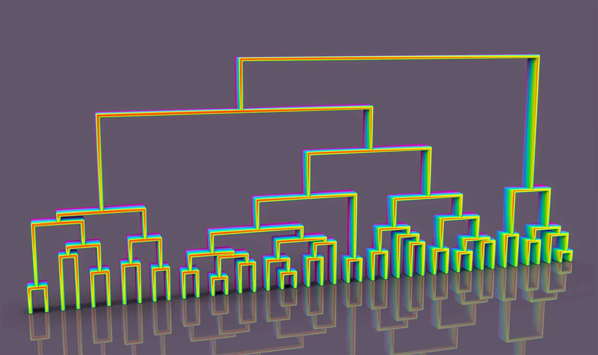
You can see how the two clusters are formed starting from the smallest clusters of two points. The vertical line that joins two clusters is the Euclidean distance between the two lines. Now let's see how dendrograms help in clustering the data. Suppose we want to divide data into two clusters. We will draw a horizontal line that passes through only two horizontal lines as shown in the figure below:

In the above case, we will have two clusters in the output. If the horizontal line crosses three vertical lines, we will have three clusters in the output. It depends upon the threshold value of the vertical distance that you chose.
Let's now see how to do agglomerative clustering using Scikit Learn library. To do so, the “AgglomerativeClustering” class from the sklearn.cluster library is used. Look at the following script:
from sklearn.cluster import AgglomerativeClustering

groups = AgglomerativeClustering(n_clusters=2, affinity=’euclidean’, linkage=’ward’)

groups .fit_predict(data)
The output looks like this
array([1, 1, 1, 1, 1, 0, 0, 0, 0, 0], dtype=int64)You can see that the first five points have been clustered together while the last 5 points have been clustered together. Let's plot the clustered points:
plt.scatter(data[:,0],data[:,1], c=groups.labels_, cmap=’cool’)
Hierarchical Clustering of Iris Data
Iris dataset contains plants of three different types: setosa, virginica and versicolor. The dataset contains labeled data where sepal-length, sepal-width and petal-length, petal-width of each plant is available. We will use the four attributes of the plants to cluster them into three different groups.
The following script imports the Iris dataset.
iris_data = pd.read_csv(‘https://raw.githubusercontent.com/uiuc-cse/data-fa14/gh-pages/data/iris.csv’)Let's see how the dataset looks like:
iris_data.head()

You can see that our dataset contains numerical values for the attributes.
Clustering is an unsupervised technique, therefore we do not require labels in our dataset. The following script removes the “species” column that contains labels, from the dataset.
iris_data.drop([‘species’], axis=1, inplace = True)Let's now see how our dataset looks like:

We will plot a pair plot to see if we can find any relation between the attributes. It can help us reduce the number of dimensions or attributes in our dataset.
Execute the following script
import seaborn as sns

sns.pairplot(iris_data)

From the output, you can clearly see that there is positive correlation between the petal-length and petal-width column which is a good indicator for clustering.
We will use only these two attributes for clustering because that way, it will be easier for us to plot the data. Execute the following script to remove the sepal-length and sepal-width attributes from our dataset.
iris_data = iris_data[[‘petal_length’, ‘petal_width’]]Let's now plot our dataset:
sns.scatterplot(x=”petal_length”, y=”petal_width”, data=iris_data)The output looks like this:

Let's now divide our data into three clusters:
from sklearn.cluster import AgglomerativeClustering

groups = AgglomerativeClustering(n_clusters=3, affinity=’euclidean’, linkage=’ward’)

groups .fit_predict(iris_data)
The output of the script above looks like this:
array([1, 1, 1, 1, 1, 1, 1, 1, 1, 1, 1, 1, 1, 1, 1, 1, 1, 1, 1, 1, 1, 1,

1, 1, 1, 1, 1, 1, 1, 1, 1, 1, 1, 1, 1, 1, 1, 1, 1, 1, 1, 1, 1, 1,

1, 1, 1, 1, 1, 1, 2, 2, 0, 2, 2, 2, 2, 2, 2, 2, 2, 2, 2, 2, 2, 2,

2, 2, 2, 2, 0, 2, 0, 2, 2, 2, 2, 0, 2, 2, 2, 2, 2, 0, 2, 2, 2, 2,

2, 2, 2, 2, 2, 2, 2, 2, 2, 2, 2, 2, 0, 0, 0, 0, 0, 0, 2, 0, 0, 0,

0, 0, 0, 0, 0, 0, 0, 0, 0, 0, 0, 0, 0, 0, 0, 0, 0, 0, 0, 0, 0, 0,

0, 0, 0, 0, 0, 0, 0, 0, 0, 0, 0, 0, 0, 0, 0, 0, 0, 0], dtype=int64)
Finally, let's plot the data points to see three clusters:
plt.scatter(iris_data[‘petal_length’] ,iris_data[‘petal_width’], c= groups.labels_, cmap=’cool’)The output of the script above looks like this:

You can see the Iris data divided into three clusters.
Conclusion
Hierarchical clustering is one of the most popular unsupervised learning algorithms. In this article, we explained the theory behind hierarchical clustering along. Furthermore, we implemented hierarchical clustering with the help of Python's Scikit learn library to cluster Iris data.
Want Help with Data Mining and Statistics projects?
Having rich experience in data mining and statistics projects, Coditude is an ideal partner for your data mining software development requirements providing flexible and cost effective engagement models.
Reach out to us to know more about how we can help you.


