In this article, we will explain how unsupervised learning techniques can help group customers based on their shopping trends. There are two main algorithms used for clustering the data: K Means Clustering and Hierarchical Clustering. In this article, we will see how K-Means Clustering can be used to divide customers with similar shopping habits into groups.
Customers Segmentation Using K Means Clustering
Machine learning algorithms can be broadly categorized into two categories: supervised and unsupervised learning. In supervised learning, the value that has to be predicted is already given. Whereas in unsupervised learning, no labeled data is available and data is grouped into clusters using statistical algorithms.
K-Means Clustering: A Simple Example
Before we move to customer segmentation, let's use K means clustering to partition relatively simpler data.
K Means Clustering algorithm performs the following steps for clustering the data:
1. The number of clusters along with the centroid value for each cluster is chosen randomly.
2. Euclidean distance between each data point and all of the centroids is calculated.
3. The data points are assigned to the cluster whose centroid has the smallest distance to the data point.
4. Centroid values for each cluster are updated by taking the mean of all the points in the cluster.
5. Steps 2, 3 and 4 are repeated until there is no difference between the previous centroid values and the updated centroid values for all the clusters.
Let's now see K-Means clustering algorithms in action.
Note: The following piece of code is executed in Jupyter Notebook.
As a first step, import the following libraries:
import pandas as pd

import numpy as np

import seaborn as sns

import matplotlib.pyplot as plt
Suppose we have a two dimensional data set with the following data points:
data = np.array([[8,12],

[12,17],

[20,20],

[25,10],

[22,35],

[81,65],

[70,75],

[55,65],

[51,60],

[85,93],])
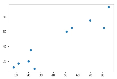
Let's plot the data points and see if we can find any clusters with the naked eye.
plt.scatter(data[:,0],data[:,1], label="True Position")
The output looks like this:
Let's manually try to divide the data points into two clusters. If you look at the data with the naked eye you can see that the five points on the bottom left of the graph belong to one cluster and the rest of the five points at the top right belong to another cluster.
Let us now try to use the K-Means Clustering algorithm to see if we made the right guess.
Execute the following script:
from sklearn.cluster import KMeans

clusters = KMeans(n_clusters=2)

clusters.fit(data)
In the script above, we import the KMeans class from the "cluster" module of the "sklearn" library. The number of clusters is passed to the "n_cluster" parameter of the constructor of the KMeans class. Next, we simply need to call the "fit()" method and pass it our data. This is all we need in order to apply the K Means clustering algorithm for clustering our data.
Now to see what centroids have finally been selected by our K Means clustering algorithm, we can use the "cluster_centers_" attribute.
The output looks like this:
[[68.4 71.6]

[17.4 18.8]]
And let's see what labels have been assigned to our data points.
print(clusters.labels_)
The output looks like this:
[1 1 1 1 1 0 0 0 0 0]You can see that the first five points belong to cluster 1 and the last 5 points belong to the second cluster with id 0. If there was a third cluster, it would have been assigned Id 2.
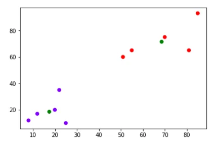
Now, to make sure that points have been clustered as we expected, let's plot the data points that belong to a different cluster in a different color. The centroids will also be printed.
plt.scatter(data[:,0], data[:,1], c=clusters.labels_, cmap="rainbow")

plt.scatter(clusters .cluster_centers_[:,0] ,clusters.cluster_centers_[:,1], color="green")
The output of the script looks like this:
From the output, you can clearly see the cluster of data points in blue and red. The green data points are the centroids for each cluster.
Customer Segmentation
In the last section, we saw how K Means clustering algorithm clusters data. Let us now move towards a more advanced section and see how K-Mean Clustering can be used to group customers into different clusters based on their shopping trends.
The dataset that we are going to use is freely available at this Kaggle Link. For the sake of experimentation, the data has is downloaded into a local drive.
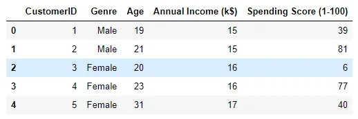
Let's first import the dataset and see how it actually looks like:
customer_data = pd.read_csv(r"D:customers.csv")

customer_data.head()
In the script above, we first import the dataset from a local drive and then print the top five rows of the data using the "head()" method of the pandas data frame. The output looks like this:
Data Analysis
Let's briefly review the columns. The CustomerID here is the ID assigned to the customer by the shopping mall. The "Genre" column contains the gender of the customer followed by the Age column which is self-explanatory. The 4th column is the "s;Annual Income (K$)"s; which contains the annual income of the customer in thousands of USD. Finally the "s;Spending Score (1-100)"s; contains the spending score of the customer, assigned by the company based on the spending habits of the customer. The higher the score, the higher is the customer spending.
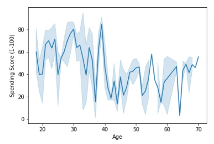
Let's now identify if there is any relationship between the different customer attributes. Let's first see if age affects the spending score. Execute the following script:
sns.lineplot(x=”Age”, y=”Spending Score (1-100)”, data = customer_data)The output looks like this:
The output suggests that there is an extremely non-linear relation between the age and the spending score. On average, people younger than 40 have a slightly higher spending score than those greater than 40.
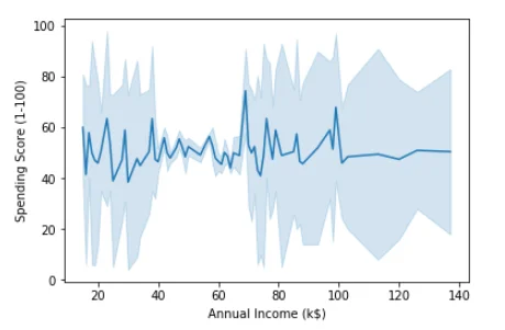
Let's plot the relationship between the annual income and spending score.
sns.lineplot(x=”Annual Income (k$)”, y=”Spending Score (1-100)”, data = customer_data)Output:
The output shows that there is no visible trend for the relation between the annual income and spending score which means that people from all the income groups have similar spending scores.
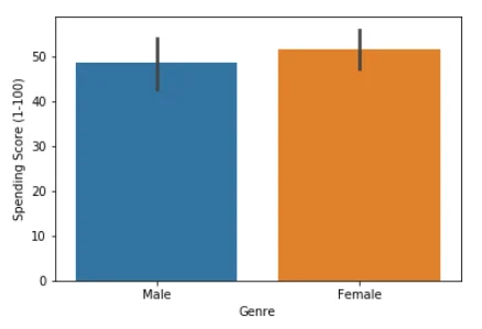
Finally, let's plot the relationship between gender and the spending score. Run the following script:
The output shows that women have a slightly higher average spending score as compared to men.
Applying K Means Clustering
In the last section, we performed exploratory data analysis of our dataset. Let us now apply K Means clustering to group the customers.
Our dataset has 5 columns and it is not easy to view data in 5 dimensions. Therefore we will perform K Means clustering on two columns only. We will use the "s;Annual Income (K$)"s; and the "s;Spending Score (1-100)"s; columns for clustering the data.
Let's remove the remaining columns from our dataset:
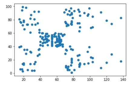
data = customer_data.iloc[:, 3:5].valuesLet's plot the dataset and see if we can manually find any clusters.
plt.scatter(data[:,0],data[:,1], label="True Position";)The output looks like this:
From the output you can see that roughly, our dataset has 5 clusters. Top left, top right, bottom left, bottom right and one in the middle. Let's see if our K Means clustering algorithm finds the same clusters.
clusters = KMeans(n_clusters=5)

clusters.fit(data)
In the script above, the number of clusters have been set to 5. Let's see what are the centroids found by our algorithms:
print(clusters.cluster_centers_)
The output looks like this:
[[25.72727273 79.36363636]

[26.30434783 20.91304348]

[88.2 17.11428571]

[86.53846154 82.12820513]

[55.2962963 49.51851852]]
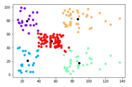
Let's now plot the data points in different colors according to their clusters
plt.scatter(data[:,0], data[:,1], c=clusters.labels_, cmap="rainbow")

plt.scatter(clusters .cluster_centers_[:,0] ,clusters.cluster_centers_[:,1], color="black")
The output of the script above looks like this:
As expected, in the output you can see that the dataset has been divided into 5 clusters: top-left(blue), top-right(light brown), bottom-left(blue), bottom-right(green) and a middle(red) clusters. You can also see the centroid for each cluster in black.
How this information is useful?
K-Means Clustering divided the customers into five groups. But how this information can be used? Let's see the output graph again.
The customers at the top right corner (light brown) are the customers with high income and high spending score. These are the customers that should be the target of the marketing campaigns as they are more likely to spend money.
The customers at the bottom right are the ones with high income but low spending score. These are the customers that spend their money carefully. Therefore, it is not advisable to waste marketing resources on such customers.
The customers in the red are the customers with average income and average spending. Though these customers are not very high spenders, they are the largest group in terms of population and therefore should be targeted while marketing. The customers in blue (bottom-left) are neither high spenders nor have high income and therefore can be left out in marketing campaigns.
Conclusion
Unsupervised learning techniques such as K Means Clustering is used to group unlabeled data. Since most of the real world data is unlabeled, clustering techniques can be extremely handy. In this article, we saw how K Means Clustering can be used to group unlabeled. We divided clustered into groups based on their shopping habits. Finally we performed an anlysis of different customer segments and extracted useful information from it.
Interested to know more?
Reinforce your B2C Marketing with intel on customer shopping habits using K-Means Clustering and execute more meaningful marketing strategies with Coditude's marketplace technology expertise.


