Predicting Customer Churn using Machine Learning Models

The Dataset

The dataset that we used to develop the customer churn prediction algorithm is freely available at this Kaggle Link. The dataset consists of 10 thousand customer records. The dataset has 14 attributes in total. First 13 attributes are the independent attributes, while the last attribute “Exited” is a dependent attribute. We downloaded the data in CSV format to our local directory.

It is important to mention that the dataset for the first 13 attributes is collected 6 months prior to collecting the dataset for the 14 column. This is because, the “Exited” column contains information on whether or not the customer exited the bank, 6 months after collecting the data for the first 13 attributes.

Customer Churn Prediction using Scikit Learn

In this section, we will explain the process of customer churn prediction using Scikit Learn, which is one of the most commonly used machine learning libraries. We will follow the typical steps needed to develop a machine learning model. We will import the required libraries along with the dataset, we will then perform data analysis followed by the preprocessing, and we will then train different machine learning algorithms on the data. Finally, we will evaluate the performance of the algorithms to see which algorithm yields the highest accuracy for customer churn prediction task.

Importing Required Libraries and Dataset

We used Python libraries for the analysis of our dataset as well as for training the machine learning models. To import the dataset we used the Pandas library. For visualizing the dataset we used Searborn library and finally to train machine learning algorithms we used Scikit learn library.

The following script imports the libraries that we are going to use to preprocess and analyze our data.

import pandas as pd

import numpy as np

import seaborn as sns

Next, we need to load the dataset into our application. The following script does that:

client_dataset = pd.read_csv(r’D:/Churn_Modelling.csv’)

Dividing Data into Training and Test Sets

Enough of the preprocessing, now we need to divide our data into training and test sets. The machine learning algorithms will be trained on the training set and will be evaluated on the test sets. But before that, let's divide our data into labels and feature set.

dataset_features = client_dataset.drop([‘Exited’], axis=1)

dataset_labels = client_dataset[‘Exited’]

In the feature set, we have all the columns except the “Exited” since the values in the “Exited” column are to be predicted. On the other hand, the label set will only contain the “Exited” column.

Now, let's divide our data into training and test set. Our test will consist of 20% of the total dataset.

from sklearn.model_selection import train_test_split

train_features, test_features, train_labels, test_labels = train_test_split(dataset_features, dataset_labels, test_size=0.2, random_state=21)

Training and Evaluation of Machine Learning Models

We divided our data into training and test set. Now is the time to create machine learning models and evaluate the performance.

We will use the three most commonly used machine learning algorithms: Random Forest, Support Vector Machines and Logistic Regression to train our models.

Random Forest

The following script trains the model using Random Forest algorithm:

from sklearn.ensemble import RandomForestClassifier as rfc

rfc_object = rfc(n_estimators=200, random_state=0)

rfc_object.fit(train_features, train_labels)

predicted_labels = rfc_object.predict(test_features)

There are several metrics to evaluate the performance of a classification algorithm. The most commonly used metrics are precision and recall, F1 measure, accuracy and confusion matrix. The Scikit Learn library contains classes that can be used to calculate these metrics. Execute the following script:

from sklearn.metrics import classification_report, confusion_matrix, accuracy_score

print(classification_report(test_labels, predicted_labels))

print(confusion_matrix(test_labels, predicted_labels))

print(accuracy_score(test_labels, predicted_labels))

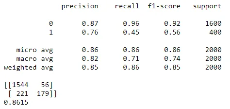
The output looks like this:

From the output, it is visible that the Random Forest achieves an accuracy of 86.15% for customer churn prediction.

Support Vector Machines

The following script trains the model using support vector machines:

from sklearn.svm import SVC as svc

svc_object = svc(kernel=’rbf’, degree=8)

svc_object.fit(train_features, train_labels)

predicted_labels = svc_object.predict(test_features)

The following script evaluates the performance of the SVM model.

print(classification_report(test_labels, predicted_labels))

print(confusion_matrix(test_labels, predicted_labels))

print(accuracy_score(test_labels, predicted_labels))

The output looks like this:

SVM achieves an accuracy of 80% for customer churn prediction.

Exploratory Data Analysis

As a first step, we need to explore our dataset and see if we can find any patterns. Let's first see the first five records in the dataset using the Head() method.

client_dataset.head()

The output of the above script looks like this:

You can see the 14 columns in our dataset. If we look at the columns carefully, we will find that there are a few columns that have no effect on whether or not a customer leaves the bank in 6 months. For instance, the first column "RowNumber" is totally random and has no effect on customer churn. Similarly, the columns "CustomerId" and "Surname" also do not have any effect on customer churn. After all, nobody leaves a bank because his Surname is XYZ. The rest of the columns such as Gender, Age, Tenure, Balance, etc. can have some sort of impact on customer churn.

Therefore, we will remove the columns "Number", "CustomerId" and "Surname" from the dataset using the following script:

client_dataset.drop([‘RowNumber’, ‘CustomerId’, ‘Surname’], axis=1, inplace = True)

Now, let's again see the first five records using the Head()method:

client_dataset.head()

You can now see that we don't have "Number", "CustomerId" and "Surname" columns in the dataset.

Next, to see the statistical details of the numeric columns in our dataset, we can use the describe() function as shown below:

client_dataset.describe()

In the output, you will see the statistical details of the data including mean, count, standard deviation, quartile etc. The output looks like this:

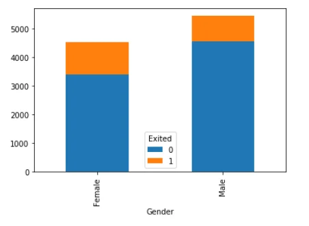
Now we have an overview of how our dataset looks like. Let's try to find the relation between individual columns and the output. Let's see if gender has any effect on customer churn. Execute the following script.

counts = client_dataset.groupby([‘Gender’, ‘Exited’]).Exited.count().unstack()

counts.plot(kind=’bar’, stacked=True)

From the output, it seems that the ratio of customers leaving the bank among females is higher than the males. Let's verify this. Execute the following script:

print(counts)

The output looks like this:

Exited 0 1

Gender

Female 3404 1139

Male 4559 898

It is evident from the output that 25% of the female customers are likely to leave the bank while in males, the percentage is 16.45%

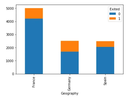
Let's now, find the relationship between the geography of the customer and the customer churn.

counts = client_dataset.groupby([‘Geography’, ‘Exited’]).Exited.count().unstack()

counts.plot(kind=’bar’, stacked=True)

The output shows that the ratio of customer churn is highest among the German customers while lower among the French customers. To further verify this fact, we can see the numbers. Execute the following script:

print(counts)

Exited 0 1

Geography

France 4204 810

Germany 1695 814

Spain 2064 413

The numbers show that France 16.15% of the French customers leave the bank, while the number is 32.44% for Germany and 20.29% for Spain.

Enough of the data analysis. Let's now preprocess our data and convert it into a format that the machine learning algorithms can work with.

In fact, we do not even need three columns to implement one hot encoding. Rather we can use two columns. For instance, we can add columns for Germany and Spain and if we want to add 1 for France, we can simply add 0 for both Germany and Spain columns which will actually mean that the Country is France, without having to add a column for France. This is done in order to avoid dummy variable trap.

The following script removes the categorical columns “Geography” and “Gender”.

tempdata = client_dataset.drop([‘Geography’, ‘Gender’], axis=1)

The following script creates one hot encoded columns for “Geography” and “Gender”.

Geography = pd.get_dummies(client_dataset.Geography).iloc[:,1:]

Gender = pd.get_dummies(client_dataset.Gender).iloc[:,1:]

Next, we need to concatenate or combine our original data set with the one hot encoded vectors. The following script does that:

client_dataset = pd.concat([tempdata,Geography,Gender], axis=1)

Now, if we look at our dataset, we will see the one hot encoded vectors in our dataset. Execute the following script to do so:

client_dataset.head()

In the dataset, the one hot encoded columns can be seen for “Geography” and “Gender” at the end.

Logistic Regression

The following script trains the model using logistic regression:

from sklearn.linear_model import LogisticRegression

lr_object = LogisticRegression()

lr_object.fit(train_features, train_labels)

predicted_labels = lr_object.predict(test_features)

The following script evaluates the performance of the logistic regression model.

print(classification_report(test_labels, predicted_labels))

print(confusion_matrix(test_labels, predicted_labels))

print(accuracy_score(test_labels, predicted_labels))

The output looks like this:

The logistic regression model achieves an accuracy of 78.5%.

Conclusion

Machine learning and deep learning approaches have recently become a popular choice for solving classification and regression problem. In this article, we explained how we can create a machine learning model capable of predicting customer churn. We tried three models and the results showed that the Random Forest algorithm performs best with an accuracy of 86.15%.

Interested to know more?

Artificial Intelligence and Machine Learning enabled customer churn analysis and predictions can help you respond accordingly to the tangible and intangible effects on the organization and develop business strategies accordingly. Drop a note to know more about our AI and ML expertise.