Text classification is defined as the process of classifying textual data into one of the predefined categories. Text classification has a wide spectrum of applications ranging from sentimental analysis to ham and spam message classification.

Text classification is defined as the process of classifying textual data into one of the predefined categories. Text classification has a wide spectrum of applications ranging from sentimental analysis to ham and spam message classification.
Both rule-based and statistical approaches have been used for text classification. Rule-based approaches involve rules based on keyword supporting, named entity recognition and parts of speech tagging. On the other hand, statistical approaches involve machine learning and deep learning.
In this article, we will see how a deep learning approach can be used to solve the task of text classification. We will use multilayer densely connected neural network, implemented in Keras Tensorflow Library, to classify text into predefined categories.
Problem Definition and Dataset
The problem that we will solve is the classification of public sentiment about six US airlines into three categories: positive, neutral and negative. The dataset is freely available at this GitHub link. The data has been collected from Twitter and has been manually annotated with the sentiment. Since the category that we want to assign to the input text is already known, text classification can be categorized as a supervised learning problem.
To solve this problem, we performed standard steps required to implement a deep learning solution.
Importing Required Libraries
The first step, as always is to import the required libraries. Execute the following script:
import numpy as np
import pandas as pd
import re
import nltk
import matplotlib.pyplot as plt
%matplotlib inline
from keras.models import Model
from keras.layers import Input, LSTM, GRU, Dense, Embedding
from keras.preprocessing.text import Tokenizer
from sklearn.preprocessing import LabelBinarizer
from keras.layers import Activation, Dropout
from keras.models import Sequential
In the script above, we imported various libraries that we need to develop the system. We will see the use of these libraries in later sections.
Importing the Dataset
The next step is to import the dataset, to do so, we used the “read_csv()” function of the Pandas library. The function takes the path to the data file as a parameter. The following script imports the dataset:
twitter_dataset = pd.read_csv(“https://raw.githubusercontent.com/kolaveridi/kaggle-Twitter-US-Airline-Sentiment-/master/Tweets.csv”)
Exploratory Data Analysis
Before feeding data into a deep learning or machine learning algorithm, it is always a good practice to analyze the dataset to find any patterns.
Let’s first see the size of our dataset:
twitter_dataset.shape
In the output, you should see (14640,15) which means that our data has 14640 records where each record has 15 attributes.
Let’s see how our dataset actually looks:
twitter_dataset.head()
A screenshot of the output is as follows:

The dataset has a column “airline_sentiment” which contains the sentiment of the tweet. This column contains the class, label or the output that we want to predict. If you scroll the above data frame to the right, you should see “text” column as shown below:

The “text” column contains tweets that we will classify as positive, neutral or negative.
Before plotting any graph, for a better view, we increase the default graph size with the following script:
plot_size = plt.rcParams[“figure.figsize”]
print(plot_size[0])
print(plot_size[1])
plot_size[0] = 10
plot_size[1] = 8
plt.rcParams[“figure.figsize”] = plot_size
In the script above we change the default plot size from 6, 4 to 10,8 which means that our new plots will be 10 inches wide and 6 inches high.
Let’s draw a pie chart that shows the share of each sentiment among the dataset.
twitter_dataset.airline_sentiment.value_counts().plot(kind=’pie’, autopct=’%1.0f%%’)
The output looks like this:
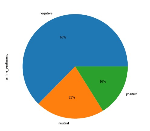
You can see from the output that 63% of all the tweets have negative sentiments, 21% have a neutral sentiment, while only 16% have positive sentiment. This shows that our dataset is not equally distributed with respect to the output.
As a final data analysis step, we will see the distribution of tweets amongst different airlines, along with the share of each sentiment. Execute the following script:
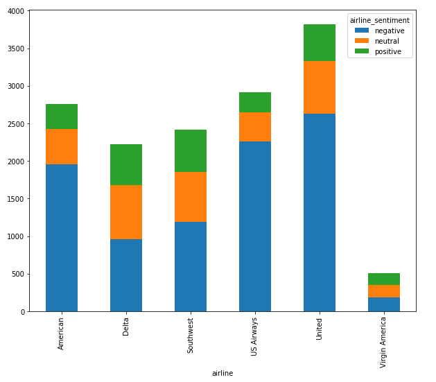
From the output, you can see that the ratio of negative tweets is higher than neutral and positive tweets for almost all the airlines.
Dividing Data Into Training and Test Sets
Before we feed our data into Keras deep learning algorithms, we divided our data into training and test sets as shown below.
X = twitter_dataset.iloc[:, 10].values
y = twitter_dataset.iloc[:, 1].values
The “iloc” function takes the index that we want to filter from our dataset. Since our feature set will consist of tweet text, which is the 11th column, we passed 10 to the first iloc function. Since column index starts from 0, therefore the 10th index corresponds to the 11th column. Similarly, for labels, we pass the 1st index.
Now variable X contains our feature set while the variable y contains our labels or the output.
Text Cleaning
Tweets contain many special characters such as @, #, – etc. Similarly, there can be many empty spaces. These special characters and empty spaces normally do not help in classification, therefore we clean our text before using it for deep learning purposes.
The following script performs text cleaning tasks.
cleaned_tweets = []
for text in range(0, len(X)):
# Remove all the special characters
cleaned_tweet = re.sub(r’\W’, ‘ ‘, str(X[text]))
# remove all single characters
cleaned_tweet = re.sub(r’\s+[a-zA-Z]\s+’, ‘ ‘, cleaned_tweet)
# Remove single characters from the start
cleaned_tweet = re.sub(r’\^[a-zA-Z]\s+’, ‘ ‘, cleaned_tweet)
# Substituting multiple spaces with single space
cleaned_tweet= re.sub(r’\s+’, ‘ ‘, cleaned_tweet, flags=re.I)
# Removing prefixed ‘b’
cleaned_tweet = re.sub(r’^b\s+’, ”, cleaned_tweet)
# Converting to Lowercase
cleaned_tweet = cleaned_tweet.lower()
cleaned_tweets.append(cleaned_tweet)
X = cleaned_tweets
The script above removes all the special characters from the tweets, then removes single spaces from the beginning. Then all the multiple spaces, generated as the result of removing special characters, are removed. Finally, for the sake of uniformity, all the text is converted to lower case. Regular expressions are used in the above script for text cleaning tasks.
Dividing Data into Training and Test Sets
Before we proceed further, we need to divide our data into a training and test set. To divide the data into training and test set, we used the “train_test_split()” function from the “Sklearn.model_selection” module. The function takes features set as a first parameter, and the label set as the second parameter. Furthermore, the value specified in fractions for the “test_size” corresponds to the percentage of data we want to reserve for the test size. We used a test size of 0.2, therefore our test size contained 20% of the data.
from sklearn.model_selection import train_test_split
X_train, X_test, y_train, y_test = train_test_split(X, y, test_size=0.2, random_state=42)
Converting Text to Numbers
Statistical approaches like machine learning and deep learning work with numbers. However, the data we have is in the form of text. We need to convert the textual data into the numeric form. Several approaches exist to convert text to numbers such as bag of words, TFIDF and word2vec.
To convert text to numbers, we can use the “Tokenizer” class from the “keras.preprocessing.text” library. The constructor for the “Tokenizer” class takes “num_words” as a parameter which can be used to specify the minimum threshold for the most frequently occurring words. This can be helpful since the words that occur less number of times than a certain threshold are not very helpful for classification. Next, we need to call the “fit_on_text()” method to train the tokenizer. Once we train the tokenizer, we can use it to convert text to numbers using the “text_to_matrix()” function. The “mode” parameter specifies the scheme that we want to use for the conversion. We used TFIDF scheme owing to its simplicity and efficiency. The following script converts, text to numbers.
vocab_size = 1000
tokenizer = Tokenizer(num_words=vocab_size)
tokenizer.fit_on_texts(X_train)
train_tweets = tokenizer.texts_to_matrix(X_train, mode=’tfidf’)
test_tweets = tokenizer.texts_to_matrix(X_test, mode=’tfidf’)
Our labels are also in the form of text e.g. positive, neutral and negative. We need to convert it into text as well. To do so, we used the “LabelBinarizer()” from the “sklearn.preprocessing” library.
encoder = LabelBinarizer()
encoder.fit(y_train)
train_sentiment = encoder.transform(y_train)
test_sentiment = encoder.transform(y_test)
Training the Neural Network
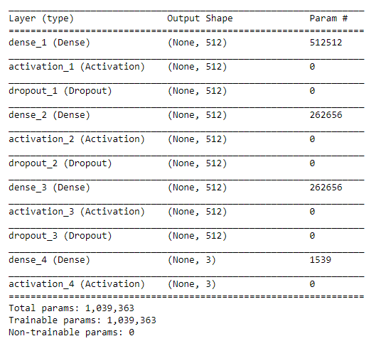
We have the data set in the form that can be used to train the neural network. We will use a neural network with three layers to learn the model that will be able to classify the public sentiment into one of the three categories. Each layer of the neural network will have 512 nodes. There is no hard and fast rule as to how much nodes or layers should be there in a neural network. It is all about trying and see which works best for you. Also, we used a 0.3 dropout rate which means that 30% of the nodes in our neural network will be forgotten in the next learning iteration. This is done in order to avoid overfitting. The activation function we used is rectified linear unit (ReLU). The number of iterations used to train the algorithm was 20. Again, it was randomly chosen. You can play around with the number of nodes, layers, the dropout and number of epochs to see if you get better results. The following script trains the algorithm:
model = Sequential()
model.add(Dense(512, input_shape=(vocab_size,)))
model.add(Activation(‘relu’))
model.add(Dropout(0.3))
model.add(Dense(512))
model.add(Activation(‘relu’))
model.add(Dropout(0.3))
model.add(Dense(512))
model.add(Activation(‘relu’))
model.add(Dropout(0.3))
model.add(Dense(num_labels))
model.add(Activation(‘softmax’))
model.summary()
model.compile(loss=’categorical_crossentropy’,
optimizer=’adam’,
metrics=[‘accuracy’])
model_info = model.fit(train_tweets, train_sentiment,
batch_size=batch_size,
epochs=20,
verbose=1,
validation_split=0.1)
The script first displays the summary of the model as shown below:
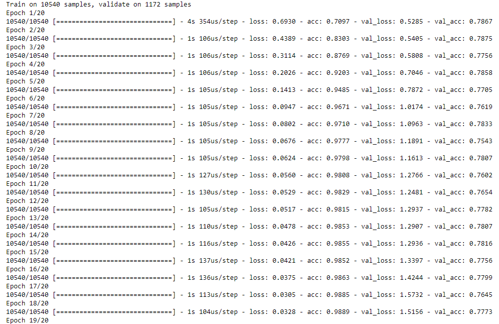
The algorithm training phase looks like this:
Evaluating the Algorithm
As the last step, we evaluate the performance of our algorithm on the test set using the following script:
result = model.evaluate(test_tweets, test_sentiment,
batch_size=batch_size, verbose=1)
print(‘Test accuracy:’, result [1])
The accuracy achieved by the model is 77.35% as shown in the output:
In this article, we explained the process of text classification using the neural network with the Keras tensorflow library. Our algorithm achieves an accuracy of 77.35% percent which is not excellent, however, given the number of records, the accuracy achieved by the system is still not bad. To further improve the accuracy, we can try a different number of layers, drop out, epochs and activation.
With customer facing businesses becoming more and more competitive, by leveraging texts and social media posts, companies can reinforce can their customer retention strategies and improve their satisfaction levels and add value to their brand. VSH’s data scientists have experience in data processing, analysis, texts cleansing and natural language processing (NLP). Drop a note to schedule an introductory call with our experts.


